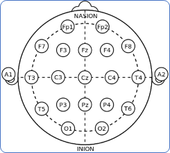
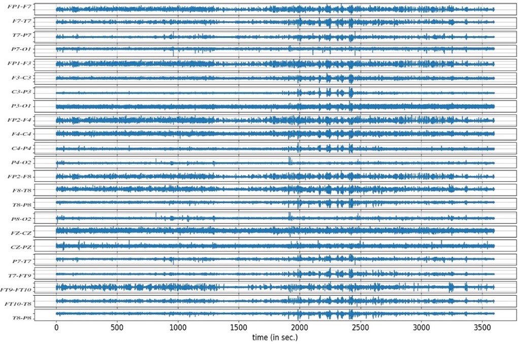
Each EEG recording had a 16-bit resolution and was sampled at 256 Hertz. Signals were simultaneously collected on 23 separate channels (FP1-F7, F7-T7, T7-P7, P7-O1, FP1-F3, F3-C3, C3-P3, P4-O2, FP2-F8, F8-T8, T8-P8, P8-O2, FZ-CZ, CZ-PZ, P7-T7, T7-FT9, FT10-T8, and T8-P8). The letter notations are P: frontopolar, F: frontal, T: temporal, O: occipital, C: central, and P: parietal. The recordings make use of the international 10-20 electrode positions system. This system uses specific landmarks on the head, such as the nasion (the bridge of the nose) and the inion (the prominent bump at the back of the skull), as reference points for electrode placement. The system divides the scalp into regions, with specific electrode placements at each location. The name "10-20" refers to the fact that the distance between adjacent electrodes is either 10% or 20% of the total front-to-back or right-to-left distance of the skull. Odd numbers (1,3,5,7) refer to the left side, while even numbers (2,4,6,8) refer to the right side of the brain. The midline electrode is indicated by the Z which is the reference electrode.

Like any neurological examination, when recording EEG, we compare the left part of the brain with the right side of the brain. The electrode,e.g., P3-O1 is placed on the left parasagittal which is the central parietal area of the brain, and the electrode e.g., P8-O2 is placed on the right parasagittal area, then we compare the left temporal with the right temporal part of the brain. We can see some channels have slow activity (C3-P3, etc), i.e. the number of waves per second is fewer compared with other channels of the brain. If these waves are less, there may be some abnormal activity in the brain. We cannot point a finger at the exact specific generator of that abnormality just from the scalp recording as spatial information is indeed lost as the electrical signals originating from the brain have to pass through the skull and other tissues before reaching the electrodes on the scalp. This can result in a blurring of the signals, making it difficult to accurately localize the sources of neural activity. Additionally, a variety of noise sources, such as electrical interference from external sources and physiological aberrations such as eye blinks, muscle contractions, and heartbeats, can greatly affect the quality of EEG data. The underlying brain signals that are of importance can be distorted or hidden by these kinds of noise, making it difficult to interpret EEG recordings precisely.

We need to clean and preprocess the EEG data in order to get beyond these limitations. Furthermore, more sophisticated analysis methods like time-frequency analysis and machine learning algorithms can aid in making it easier to differentiate between irrelevant brain activity and signals.

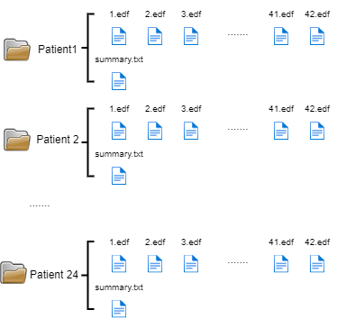
To enable the use of the EEG signals for model training, the data needs to be load, read, concatenated in a big file for every patient and stored for posterior use.

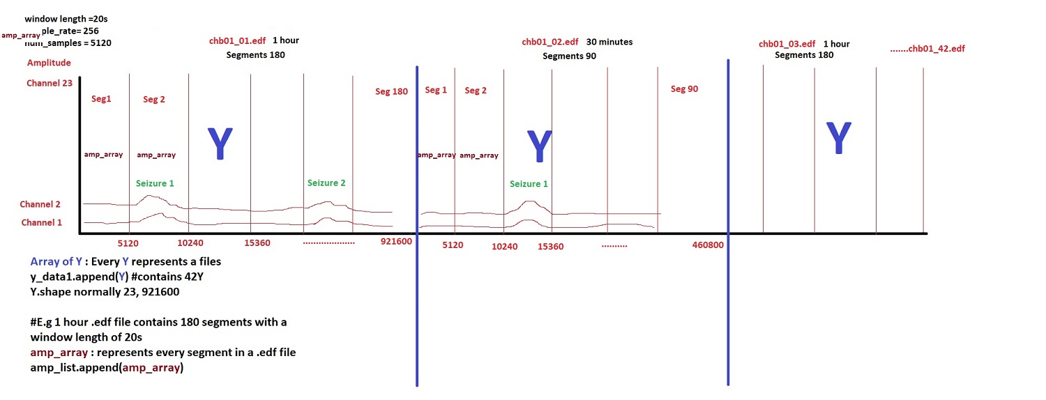
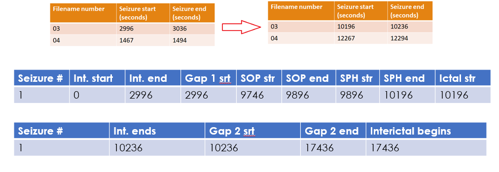
The following picture shows the concatenation of all edf files along a big array in order to be able not only to use them for model learning but also for segmenting the data by window length in seconds. This segmentation is important to try different window lengths associated with labeling of the data.